Timing Attacks using Machine Learning

Most timing attacks fail because the timing differences are too small and the noise is too big.
Naive statistical measures like mean, median or percentile neglect the inner structure of the data and perform poorly in difficult cases. In this article we will analyze and model timing attacks, enabling us to apply machine learning techniques and power up timing attacks as we knew them.

Introduction to Timing Attacks

Explaining timing attacks in three sentences: A Hacker can infer that a password starts with “S” because the server responds to ‘SXXXX’ a tiny bit slower than to ‘AXXXX’, ‘BXXXX’, … . This is caused by the implementation of a string-compare function, that iterates over the strings character by character and returns upon finding the first characters that don’t match. Using this principle the attacker is able to reconstruct the whole password character by character.

In this article we will exemplify timing attacks with finding out a password, but different objectives are possible like inferring a web-token or crypto secret.

Mathematically, we can compare the run times for finding out the whole password of length n:
Brute Force: $O(|A|^n)$
Timing Attack: $O(n\times|A|)$
where $|A|$ is the amount of all possible characters in a password.

Enough of the basics!
We will make measurements, visualize the data and construct a model to describe the observations.

Analyzing: The slow string compare

Before we will analyze the fastest string-compare function that python has to offer, let’s look at a slower string-compare function:

TRUE_PW = "SuPerDupeRStrongPassword"
def str_compare_slow(str1, str2):
    counter = 0
    while counter < len(str1) and counter < len(str2):
        if str1[counter] == str2[counter]:
            counter = counter + 1
        else:
            return counter

Firstly, we want to measure string-compare timings and visualize them, in order to understand and model the data.

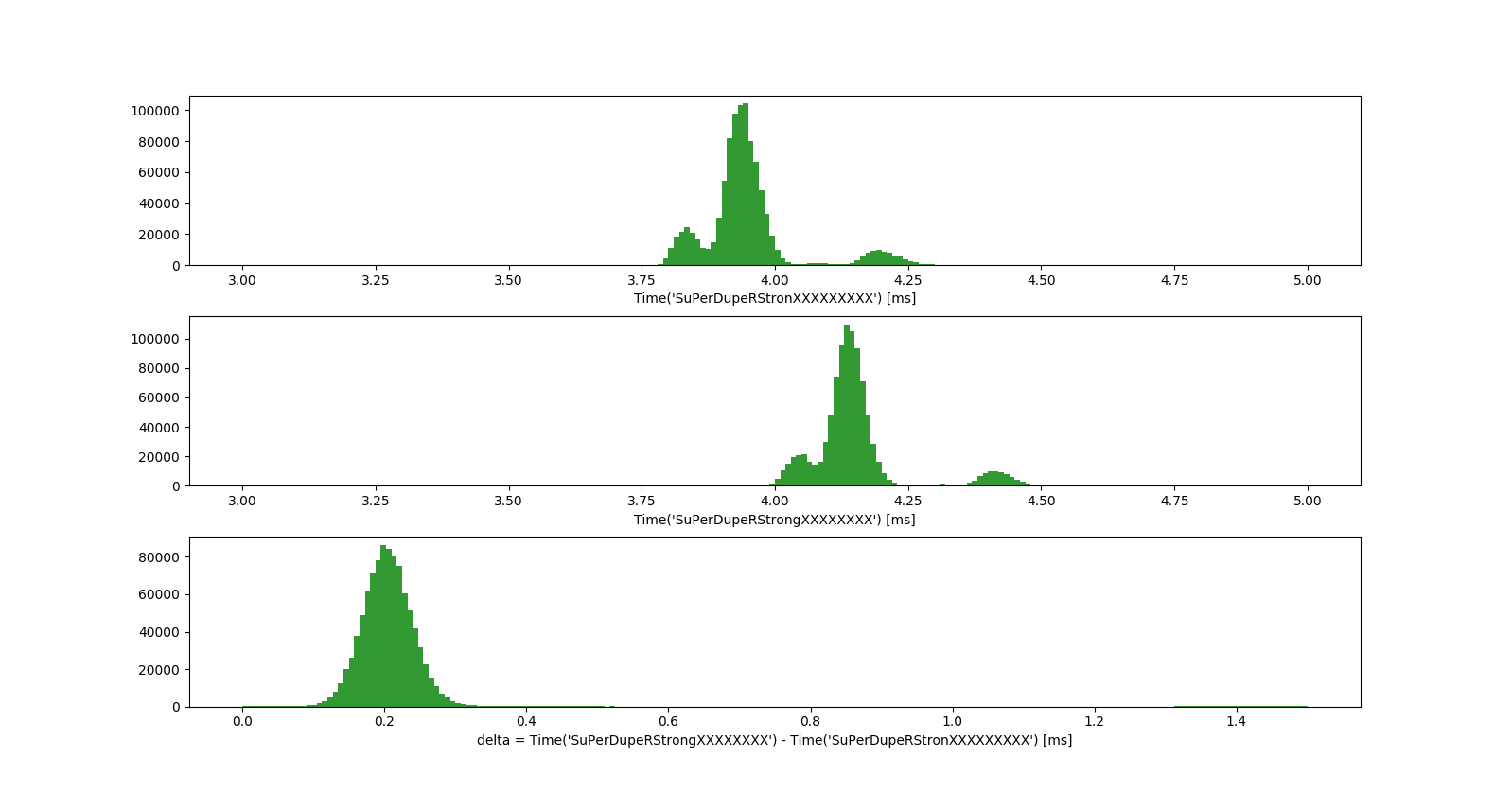
We can observe the timing distribution of the ‘string_compare_slow’ function in the first two rows. The distributions show a big Gaussian, surrounded by smaller Gaussians which are caused by system-specific noise like scheduling delays or network-routing.
The last row shows the difference of the timing distributions, which is a simple Gaussian distribution ($\mu_\Delta=0.2$). This $\Delta$ is exactly the amount of time it takes the ‘string_compare_slow’ function to check the next correct character.
We make a very important observation here: When we measure timings, it is essential to measure a reference timing before and take the difference of the two measurements. By doing this we get can rid of complex system-specific noise and obtain a simple Gaussian distribution $\Delta$ (third row).

Formalizing our observations - we define the response time of the server when the first $k-1$ characters are correct as $T_k$:
$T\_{k} = T\_{k-1} + \Delta\_k$
Hence,
$\Delta\_k = T\_{k} - T\_{k-1}$
where
$\Delta\_k \sim \begin{cases} \mathcal{N}(\mu , & \nu), & \text{if k'th character is correct} \\ \mathcal{N}(0 , & \nu'), & \text{if k'th character is incorrect} \end{cases}$
So in each iteration step, for each candidate character we make a reference time measurement $T_{k-1}$ and subtract it from the time measurement of the candidate character $T_{k}$ to obtain $\Delta_k$.
If the k’th character is incorrect, the time difference $\Delta_k$ should on average be zero. On the other hand if the k’th character is correct, we expect to measure an average delay $\mu > 0$.

So when we measure timing differences $\Delta_k$ for the next character in the password, we get a mixture of two Gaussian distributions, one being generated by the incorrect characters and one being generated by the next correct password character:

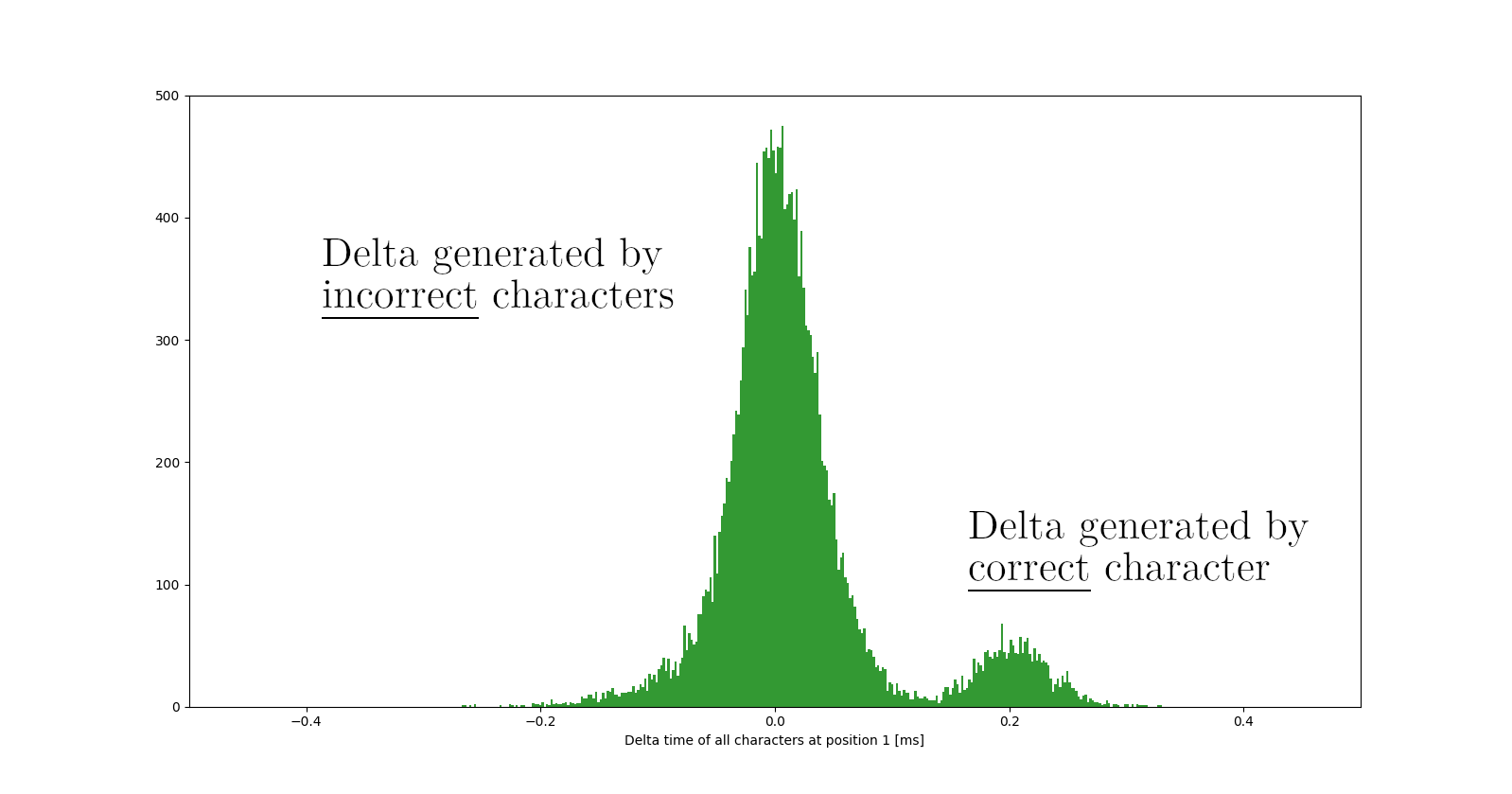
Thanks to a machine learning technique called Gaussian Mixture Modelling we can automatically compute the mean and the variance of these two Gaussians, and compute for each character the probability that it was generated by $\Delta_{correct}$ or $\Delta_{incorrect}$. By doing this, we can not only determine the next correct character but also detect if we have chosen a bad character in an iteration step before, but we will come to that later.

You might think - “Why make it so complicated if I can just take the mean for each character and pick the character with the biggest mean as the next character of the password?”
Well, if we look at faster string-compare functions, taking the mean will not suffice anymore since the variance of the data is bigger than the separation of the means.
This means that most of the times we will pick a wrong character, because the data is too noisy.

Let’s look at this case where the time differences are so small, such that the Gaussians ‘melt’ together.

The fast string compare and Gaussian Mixture Models

To visualize why median, mean or percentile fail as robust metrics to determine the next correct character, let’s look the fastest string-compare function that python has to offer:

def str_compare_fast(str1, str2):
    return str1 == str2

Measuring the time differences caused by this fast string-compare function:

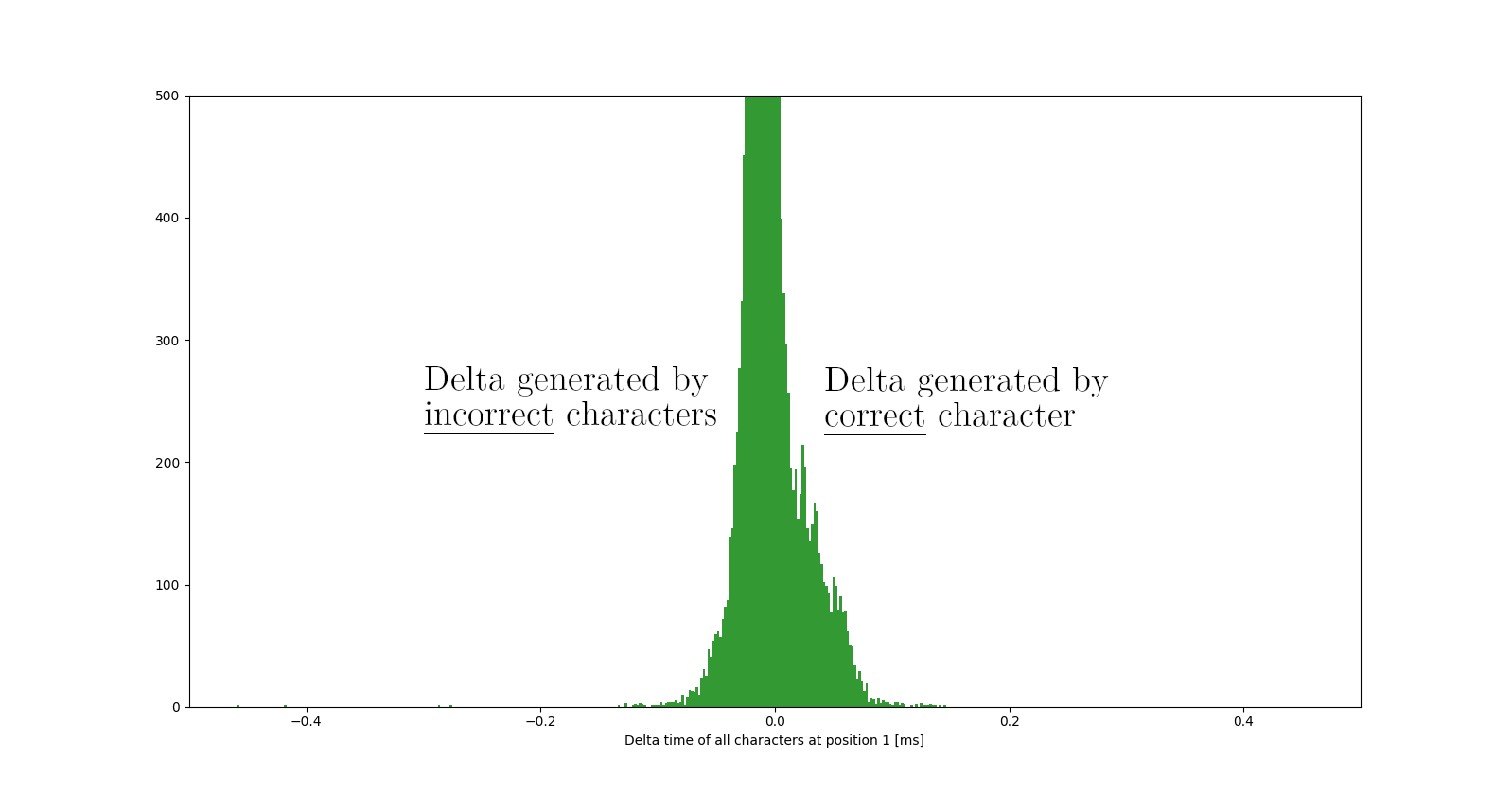
As we can see, the distributions are not well separated and naive metrics like mean, median or percentile fail most of the times, since the data is pretty noisy.

But since we know that the data is generated from two Gaussians, we can leverage Gaussian Mixture Models to compute the two most likely Gaussians that generated the data.

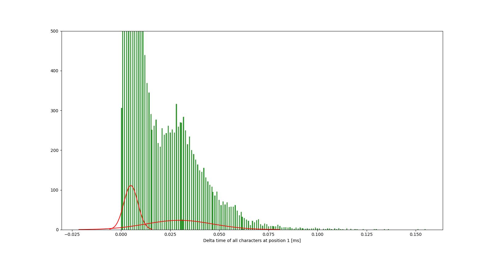
By modelling the data as a Gaussian Mixture Model, timing attacks become more resistant to noisy measurements and we are able to compute the probability of a character to be correct.
Assigning probabilities enables us to measure a confidence of the correctness of a selected character as well as detection of wrongly chosen characters.

So the algorithm to decide on the next character works as follows:
1) Build Gaussian Mixture Models (two Gaussians) from the timing differences
2) For each character, compute the probability that its measurements were generated
by Gaussian distr. 1 or Gaussian distr. 2
3) Select character of highest probability to belong to biggest-mean Gaussian as the
next character

The next plot shows the probability that a character is correct:

The plot shows that the character “w” has the highest probability (> 0.9) to be generated from the “correct”-Gaussian. This is in fact the correct next character. The other characters fall off well, having probabilities of < 0.6.

In the case where we made a wrong decision and picked a wrong character as the next character, looking at the following plot helps us detect that:

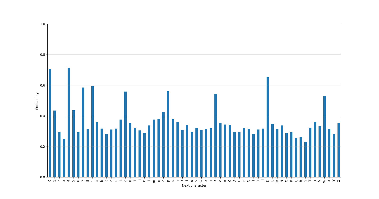
As we can see, no character is extremely likely to be generated by the “correct”-Gaussian. All characters have probabilities of < 0.8.
In our algorithm, if no character has probability of > 0.9, we will go back one step and decide on the previous character again.

The following GIF shows the execution of our algorithm including the detection of wrong choices:

If you want to see the code or implement your own timing analysis using Gaussian Mixture Models, I have compiled a small API on github here.

As we have seen, modelling the data generation and applying machine learning techniques gave us the possibility to detect wrongly chosen characters and deal with noise-intensive processes in a straight forward manner.

Define and conquer!

niknax